Mapping the Epigraphic Habit

Published: July 17, 2019

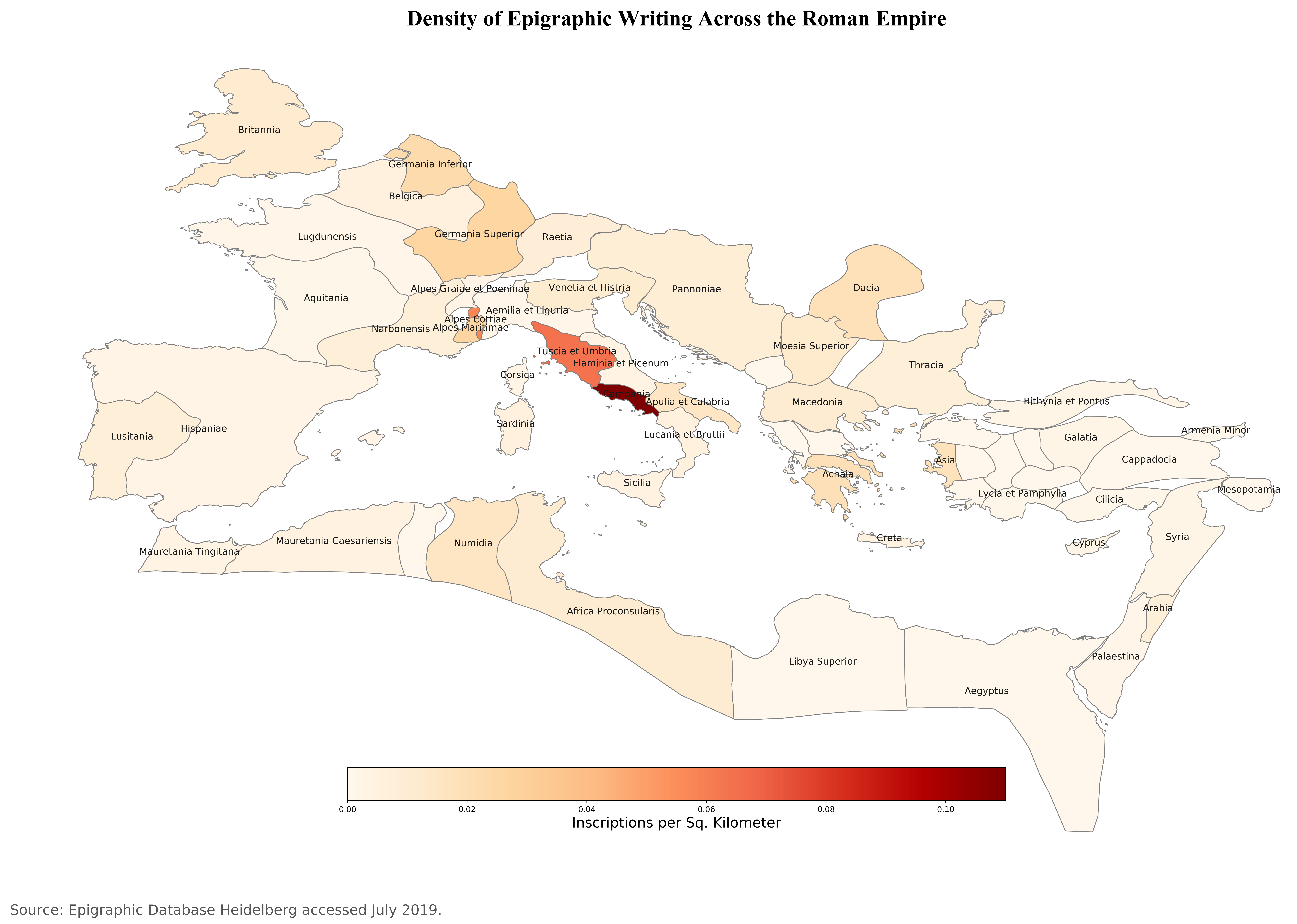
Across the Empire, Romans inscribed the significant events of their lives on stone. A record of deaths, vows to the gods, and public decrees, these inscriptions reached their highest frequency around the year 200 A.D. The map below depicts the density of inscription writing in Italy and the surrounding provinces.

png

The highest concentration of writing comes from the immediate vicinity of Rome, but epigraphy extended to Greece, Germany, Northern Africa, and parts of Asia Minor as well.

The data include all 76,652 inscriptions from the Epigraphic Database Heidelberg that indicate where the inscription was found. Wilson (2014) suggests using these inscriptions as a proxy for Roman economic activity. This map is a first stab at exploring the data to that end.

Find the source code below:

import pandas as pd
import geopandas as gpd
import matplotlib.pyplot as plt
import numpy as np

#%% Read in shapefile and inscription data

directory = ""
map_df = gpd.read_file(directory + "\\provinces\\provinces.shp")
map_df.drop_duplicates(subset=["name"], keep='first', inplace=True)
df = pd.read_csv(directory + "\\map_data.csv")
df['label'] = df['map_province']
map_df['all_names'] = map_df['name']

#%% Province & area lookups
# prov = pd.unique(map_df['name'])
# pd.DataFrame(prov).to_csv(directory + "\\provinces.csv")

# tost = map_df.copy()
# tost = tost.to_crs({'init': 'epsg:3857'})
# tost["area"] = tost['geometry'].area/10**6
# tost[['area', 'name']].to_stata(directory + "\\province_areas.dta")
#%% Merge datasets and filter out overlapping provinces. 
# Set NaN values to 0.

merged = map_df.set_index('name').join(df.set_index('map_province'))
merged.replace({'num_inscriptions': {np.nan:0}, 
	            'num_persons': {np.nan:0}, 
				'volume': {np.nan:0},
                'inscriptions_per_km': {np.nan:0}}, inplace=True)

extra = ['Thessalia', 'Hellespontus', 'Caria', 'Lydia', 'Phrygia I', 
         'Phrygia II', 'Pisidia', 'Hellespontus', 
	 'Mauretania Sitifensis', 'Praevalitana', 'Epirus Vetus']
merged = merged[merged.num_inscriptions != 0 | 
                merged.all_names.isin(extra)]

#%% Plot the map

# Set the location of the province labels
merged['coords'] = merged['geometry'].apply(lambda x: x.centroid.coords[:])
# merged['coords'] = merged['geometry'].apply(lambda x: x.representative_point().coords[:])

merged['coords'] = [coords[0] for coords in merged['coords']]

fig, ax = plt.subplots(1, figsize=(30,24))
merged.plot(edgecolor='gray', column='inscriptions_per_km', 
            ax=ax, cmap='OrRd')

# Label the provinces
for idx, row in merged.iterrows():
    if pd.notnull(row['label']):
        plt.annotate(s=row['label'], xy=row['coords'], 
		horizontalalignment='center', size=12, color='.1')


# Title and notes
ax.axis('off')  
ax.set_title('Density of Epigraphic Writing Across the Roman Empire', 
             fontdict={'fontsize': '28', 'fontweight' : '5', 
			 'fontname' : 'Times New Roman'})
ax.annotate('Source: Epigraphic Database Heidelberg accessed July 2019', 
	        xy=(0.12, 0.1),  xycoords='figure fraction', 
		horizontalalignment='left', verticalalignment='top', 
		fontsize=18, color='#555555')
   
# Add a colorbar     
vmin, vmax = 0, .11
sm = plt.cm.ScalarMappable(cmap='OrRd', 
                           norm=plt.Normalize(vmin=vmin, vmax=vmax))
sm._A = []
cb = ax.get_figure().colorbar(sm, ax=ax, orientation='horizontal', 
                             fraction=.1, shrink = .5, pad=-.1)
cb.set_label('Inscriptions per Sq. Kilometer', size=18)

fig.savefig(directory + "\\roman_inscriptions.png", dpi=400)

Sources:

Wilson, Andrew I. 2014. “Quantifying Roman Economic Performance by Means of Proxies : Pitfalls and Potential.” Edited by Francois de Callatay, 147-67. Pragmateiai. Edipuglia. https://ora.ox.ac.uk/objects/pubs:503490

Cooley, Benjamin. “Let’s make a map! Using Geopandas, Pandas, and Matplotlib to make a Choropleth map.” Medium. https://towardsdatascience.com/lets-make-a-map-using-geopandas-pandas-and-matplotlib-to-make-a-chloropleth-map-dddc31c1983d

Colin Williams

Sources: